


Modelling economies of scale

One key area in which the simulation MBT Arjun Mk.1A vs T-90MS fell short was the inability to factor in economies of scale from producing large numbers of Arjuns.

Image source: Strategy for Executives
I’ve overcome that, to an extent, by incorporating the 0.6 rule to approximate of economies of scale.
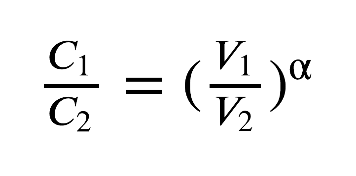
V1 is taken as initial volume and V2 is taken as cumulative volume after multiple batches have been manufactured. C1 is the cost of producing V1, and C2 is the cost of producing V2. α is a coefficient that depends on how ‘amenable’ a product / process is to economies of scale.
A value of α below 1 implies increasing economies of scale, and 0.6 is the value typically taken as rule of thumb.
In my simulation, α begins at 0.6 for the domestic product because invariably they haven’t been produced in large enough quantities for economies of scale to kick in. Over the duration of the procurement, my simulation adjusts α such that it ends up at 1, implying that there are no more economies of scale to be harnessed.
The simulation assumes that the imported product, which is invariably already in service with the manufacturing nation’s armed forces, has less scope for further economies of scale. Therefore it only permits economies of scale for 20% of the duration of procurement, with α reaching 1 at the end of that short duration.
There are more complex models for economies of scale, of course, but the 0.6 rule provides numbers that are decent enough for the purpose of these simulations.